Describing a data set
Types of variables, location, spread and graphical displays.
The type of variable drives everything
A qualitative variable is counted, a quantitative variable is measured. This distinction alone determines which summary measures can be used, which charts make sense and which tests apply.
Among quantitative variables, we further separate discrete ones, which only take isolated values, from continuous ones, which can take any value within an interval.
Location and spread
The mean is sensitive to extreme values; the median is not. For a skewed distribution or one with outliers, the median describes the center better.
Spread is described by the standard deviation around the mean, or by the interquartile range around the median. A measure of location alone never describes a data set: two data sets with the same mean may have nothing in common.

Describe before concluding
The type of variable dictates the description. A qualitative variable is described by counts and percentages. A quantitative variable is described by a measure of location and a measure of spread, always both — a mean alone says nothing.
The choice of measure depends on the shape of the distribution. If it is symmetrical, the mean and standard deviation are appropriate. If it is skewed, the mean is pulled by extreme values and becomes misleading: the median and quartiles are preferred.
Ordinal variables sit in between. Their categories are ordered, but the gaps are not measurable: nothing says that going from stage I to II is equivalent to going from II to III. Calculating their mean therefore makes no sense; they are described by counts and percentages, or by the median.
Calculating by hand
Take five blood glucose values: 4, 5, 5, 6 and 10 mmol/L. The mean is their sum divided by their number, 30 / 5 = 6. The median is the middle value once the series is sorted, here 5; with an even number of values, it is the mean of the two central values. The mode, the most frequent value, is 5. The range, the difference between maximum and minimum, is 6.
Variance measures spread around the mean: it is the mean of the squared deviations from the mean. The deviations here are −2, −1, −1, 0 and 4, their squares 4, 1, 1, 0 and 16, summing to 22. To describe a sample and estimate the population variance, one divides by n − 1 rather than n, which corrects a slight underestimate: 22 / 4 = 5.5. The standard deviation, the square root of the variance, is about 2.3 mmol/L and is expressed in the variable's unit.
The value 10 pulls the mean up but does not change the median: this is what makes the median more robust to extreme values.
Showing the data
The box plot summarises a quantitative variable at a glance. The box runs from the first to the third quartile and so contains the middle half of the values; its length is the interquartile range. A line marks the median. The whiskers extend to the most distant values lying within one and a half interquartile ranges of the box; beyond that, values are drawn individually as outliers.
In a histogram, it is the area of each bar, not its height, that is proportional to the count, which matters when classes have unequal widths. A scatter plot shows the relationship between two quantitative variables; a bar or pie chart, the distribution of a qualitative variable.
A graph can mislead. A vertical axis not starting at zero exaggerates differences; different scales on two graphs side by side distort the comparison; a percentage without its count hides the fragility of a result based on a few subjects.
The normal distribution and reference ranges
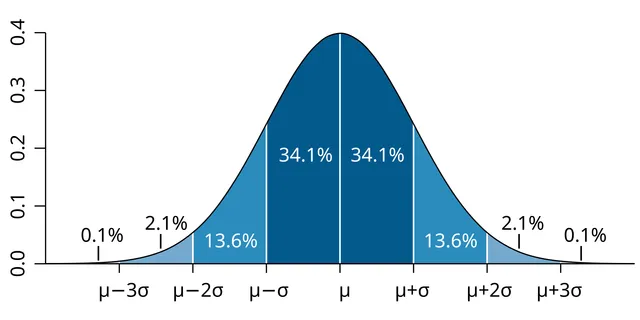
To place a value in a normal distribution, one centres and scales it: subtract the mean and divide by the standard deviation. This gives a z-score, which says how many standard deviations the value lies from the mean. About 68% of values have a z between −1 and +1, 95% between −1.96 and +1.96, and 99.7% between −3 and +3.
Children's growth charts use this principle: a height at −2 standard deviations places the child among the smallest 2 to 3% of their age.
The reference range of a laboratory test is generally defined as the interval containing 95% of healthy people. By construction, 5% of healthy people therefore have a value outside this range. On a panel of twenty independent tests, a perfectly healthy person thus has a good chance of having at least one "abnormal" result by chance alone.
Linking two variables
Pearson's correlation coefficient measures the strength of a linear relationship between two quantitative variables; it ranges from −1 to +1. Its square indicates the share of one variable's variability that is linked to the other's: a correlation of 0.5 explains only a quarter. A zero correlation means no linear relationship, not no relationship at all: a U-shaped relationship can give a coefficient close to zero.
Correlation does not prove causation. Two variables can vary together because a third influences both: this is a confounding factor. Ice cream sales and drownings rise together, because both rise with heat.
Linear regression goes further and describes the relationship with a straight line, of equation y = a + bx. The slope b indicates by how much y changes, on average, when x increases by one unit. For two qualitative variables, counts are cross-tabulated in a contingency table.
Percentages: common pitfalls
A percentage makes sense only with its denominator: "50% recovered" does not carry the same weight for two patients as for two thousand. One must also know what the percentage is of: the share of smokers among patients is not the share of patients among smokers.
Going from 10% to 15% is a rise of five percentage points, but a relative increase of 50%. Both statements are correct; the second is more impressive, and it is often the one highlighted.
Finally, pooling data can reverse a trend: a treatment can appear better in each of two subgroups and worse overall, if the subgroups are of very different sizes and severities. This is Simpson's paradox, a reminder always to ask whether the groups compared are comparable.
58 answered questions go with this chapter in the practice section.
Sources and further reading
Reference textbooks
- Daniel Schwartz, Méthodes statistiques à l'usage des médecins et des biologistes, Flammarion Médecine-Sciences.
Open access
- 2.7 Measures of the Spread of the Data — OpenStax, Introductory Statistics 2e.
Last revised : . Text licensed under CC BY-SA 4.0.