Sampling and estimation
Sampling variability, confidence interval, precision.
What a confidence interval really says
We only observe a sample, and we want to draw conclusions about a population. The gap between the two is sampling variability: it is inherent to random sampling and exists even with a perfect method. Statistics does not eliminate it; it quantifies it.
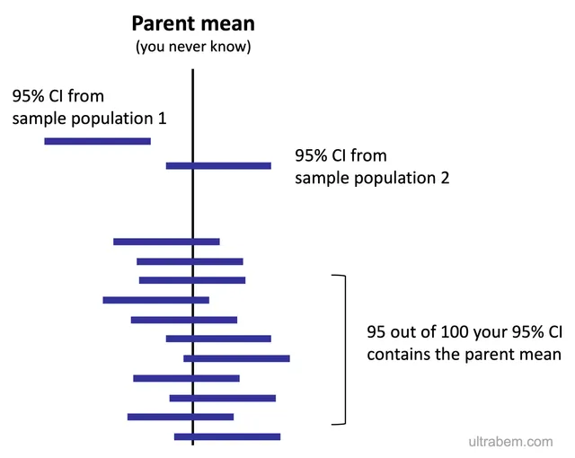
The confidence interval is that quantification. Its exact wording concerns the procedure, not the interval in front of you: if the study were repeated a large number of times, ninety-five percent of the intervals built this way would contain the true value. It also says more than a test does: the direction, size and precision of the effect, where a test only returns a yes-or-no verdict.
Its width increases with the variability of the data and decreases in inverse proportion to the square root of the sample size. Gaining a factor of two in precision therefore requires four times as many subjects — which explains the quickly prohibitive cost of studies aiming to detect small effects.

Estimating a mean, estimating a proportion
A point estimate sums up the sample in a single number: the observed mean for a quantitative variable, the observed frequency for a qualitative one. On its own, it says nothing about its own precision.
That precision is measured by the standard error, the standard deviation of the estimate from one sample to the next. For a mean, it equals the standard deviation of the data divided by the square root of the sample size. The two must not be confused: the standard deviation describes the spread of individuals, the standard error that of the mean.
With a large enough sample, the 95% confidence interval is the estimate plus or minus 1.96 standard errors. For a proportion p observed in n subjects, the standard error is the square root of p(1 − p)/n — an approximation valid when np and n(1 − p) are both at least five.
Sampling properly
The precision of an estimate depends on sample size; its accuracy depends on how the sample was drawn. Only random selection from the target population — random sampling — guarantees that every individual has the same chance of being included, and allows confidence interval calculations to apply.
Variants make it practical. Stratified sampling draws separately within subgroups — age, region — to guarantee they are represented; cluster sampling draws whole units, schools or villages, when no list of individuals exists.
A sample of volunteers, of hospital patients or of people reached online is not representative of the general population. It can yield precise estimates, but they describe a different population from the one we think we are studying.
Two standard calculations
In a sample of 100 adults, mean systolic pressure is 120 mmHg, with a standard deviation of 15 mmHg. The standard error of the mean equals the standard deviation divided by the square root of the sample size: 15 / 10 = 1.5 mmHg. The 95% confidence interval extends 1.96 standard errors either side of the mean, about 120 ± 2.9, that is from 117.1 to 122.9 mmHg.
Of 400 people surveyed, 80 smoke: the observed proportion is 20%. Its standard error is the square root of p(1 − p)/n, the square root of 0.2 × 0.8 / 400 = 0.02. The 95% interval is 20% ± 1.96 × 2%, roughly 16% to 24%.
These formulas rely on the normal approximation. For a proportion, it is acceptable when at least five subjects are expected in each category, that is n × p and n × (1 − p) both at least 5. For a mean in a small sample, 1.96 is replaced by a slightly larger value taken from Student's distribution, which depends on sample size.
Some probability distributions
The binomial distribution describes the number of successes in a series of n independent trials each having the same probability p of success: the number of boys in a sibship, the number of patients cured out of n treated. Its mean is n × p. When n is large, it approaches a normal distribution.
The Poisson distribution describes the number of rare events occurring in an interval of time or space, such as the number of cases of a rare disease per year in a region. Its mean and variance are equal.
The normal distribution is the most used, not because all biological variables are normal — many are not — but because, according to the central limit theorem, the mean of a large enough sample approximately follows a normal distribution, whatever the starting distribution. This is what justifies confidence intervals and many tests.
Precision and accuracy
An estimate can be wrong in two ways. Random error, due to sampling fluctuation, scatters estimates around the true value: it decreases as sample size increases, and the confidence interval measures it. Systematic error, or bias, shifts all estimates in the same direction: it does not decrease with sample size, and the confidence interval does not see it.
The image of a target helps to remember the difference. Shots grouped tightly but far from the centre are precise but biased; shots scattered around the centre are accurate on average but imprecise. A large biased study gives a narrow interval… around a wrong value.
Biases fall into three families. Selection bias comes from how subjects are recruited: volunteers healthier than the population, people lost to follow-up who differ from those who remain. Measurement, or information, bias comes from how data are collected: a poorly calibrated device, patients who remember their exposures better than controls. Confounding bias comes from a third factor linked both to the exposure and to the outcome.
How many subjects to include
Before a study, the number of subjects needed is calculated to have a good chance of demonstrating the effect sought if it exists. This number increases when a lower alpha risk or higher power is wanted, when measurement variability is large, and above all when the effect sought is small.
Sample size varies as the inverse of the square of the effect: to detect an effect half as large, about four times as many subjects are needed. This is why studies looking for small benefits, for example a slight reduction in mortality, include thousands or tens of thousands of patients.
A study that is too small has little chance of reaching a conclusion even if the treatment works, and its positive results, when they occur, often overestimate the effect. Recruiting patients into a study that cannot answer its question also raises an ethical problem.
Reading the interval of an effect
Often what is estimated is not a mean but an effect: a difference between two means, a relative risk, an odds ratio. The confidence interval of a difference is read against 0, the value meaning no difference; that of a ratio is read against 1. If the 95% interval contains the no-effect value, the difference is not significant at the 5% level, and vice versa: test and interval say the same thing.
Yet the interval says much more than a p-value. A relative risk of 0.80 with an interval of 0.70 to 0.91 indicates a risk reduction plausibly between 9% and 30%. A relative risk of 0.80 with an interval of 0.50 to 1.30 is compatible with a large benefit as well as with no effect, or even harm: the study has not settled the question.
To judge clinical relevance, one looks at the least favourable bound of the interval: if even that corresponds to a benefit useful to patients, the result is both significant and clinically important.
58 answered questions go with this chapter in the practice section.
Sources and further reading
Reference textbooks
- Daniel Schwartz, Méthodes statistiques à l'usage des médecins et des biologistes, Flammarion Médecine-Sciences.
Open access
- 7.2 The Central Limit Theorem for Sums — OpenStax, Introductory Statistics 2e.
- 8.1 A Single Population Mean using the Normal Distribution — OpenStax, Introductory Statistics 2e.
Last revised : . Text licensed under CC BY-SA 4.0.