Hypothesis tests and error risks
Null hypothesis, p-value, alpha and beta risks, power.
The two risks, and what p does not say
A test confronts a null hypothesis, that of no difference, with the observed data. Two errors are possible. Wrongly rejecting the null hypothesis is the alpha risk, set in advance, usually at five percent: this is the false positive. Failing to reject it when it is false is the beta risk: this is the false negative, and power is its complement.
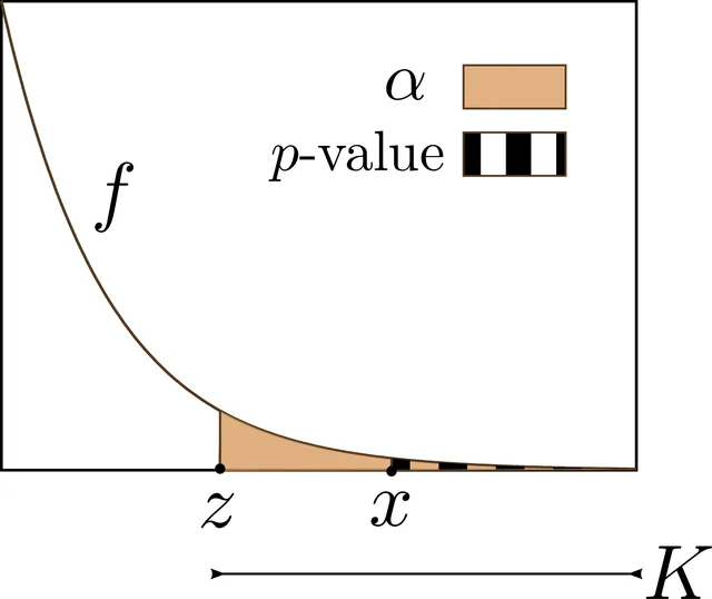
The p-value is the probability of observing a result at least as extreme if the null hypothesis were true. It is not the probability that this hypothesis is true, nor is it a measure of how large the effect is. A p of 0.04 therefore does not mean there is a four percent chance of being wrong when concluding that a difference exists.
Two consequences follow. A non-significant result does not prove there is no difference: it may simply reflect a lack of power. And a significant difference is not necessarily important: with a large enough sample, a clinically negligible gap becomes statistically significant.

How a test works
A test always follows the same steps. State the null hypothesis, H0, and the alternative; set the alpha risk before looking at the data; compute, under H0, a test statistic whose distribution is known; finally compare its value with the threshold corresponding to alpha.
If the statistic exceeds the threshold, H0 is rejected and the difference is said to be significant at level alpha. Otherwise H0 is not rejected — which is not the same as accepting it: we only conclude that the data are not enough to show a difference.
A test is two-sided when a difference in either direction is sought, one-sided when only one direction is considered. The choice is made before the analysis; switching to a one-sided test afterwards, to cross the threshold, amounts to doubling the alpha risk actually taken.
Choosing the test
The choice depends on the type of variables and the study design. To compare two proportions, use the chi-squared test, or Fisher's exact test when expected counts are small. To compare two means, use Student's t-test, which assumes a normal distribution or a large enough sample.
When measurements are paired — the same subject before and after treatment — use the paired versions of these tests, which work on individual differences and gain a great deal of power. When normality conditions are not met, non-parametric rank-based tests, such as the Wilcoxon or Mann-Whitney tests, take over.
To study the association between two quantitative variables, test the correlation coefficient. A significant correlation says nothing about the direction of the relationship, nor about whether it is causal.
A chi-square test step by step
A trial compares two treatments in 200 patients, 100 per group. There are 60 cures with treatment A and 40 with treatment B, 100 cures in total. The null hypothesis is that the cure rate is the same in both groups.
Under this hypothesis, half of each group is expected to be cured, since 100 of 200 patients were cured: the expected count for each cell equals its row total times its column total, divided by the overall total, 100 × 100 / 200 = 50. The four expected cells are therefore 50.
The chi-square statistic adds, for each cell, the square of the difference between observed and expected divided by expected: (60 − 50)² / 50 = 2 for each of the four cells, 8 in total. A table with two rows and two columns has one degree of freedom; the 5% threshold is 3.84. Since 8 exceeds 3.84, the null hypothesis is rejected: the difference is significant. The test is valid only if all expected counts are large enough, usually at least 5.
Paired or independent samples
The choice of test depends first on the study design. When two groups of different subjects are compared, the samples are independent. When the same subjects are measured twice — before and after treatment, right and left eye — or subjects are matched one to one, the samples are paired: each subject serves as their own control, which removes much of the between-person variability and makes the test more powerful.
To compare two means, Student's t-test for independent samples or for paired samples is used; if normality conditions are not met, their rank-based non-parametric equivalents are the Mann-Whitney test and the Wilcoxon test. For two paired proportions, McNemar's test is used.
To compare more than two groups, pairwise tests are not chained, which would multiply the risk of error: an analysis of variance is used, or its non-parametric equivalent, the Kruskal-Wallis test, which first tests globally whether any difference exists.
The trap of multiple testing
Each test carried out at the 5% level has a one-in-twenty chance of wrongly concluding that there is a difference. If twenty independent tests are run on data where nothing is true, the probability of getting at least one significant result by chance is 1 − 0.95 to the power 20, about 64%.
Several remedies exist. The simplest, the Bonferroni correction, divides the threshold by the number of tests: for ten tests, each must reach p < 0.005. Above all, a trial must define a primary endpoint in advance, on which the conclusion rests; the other analyses are exploratory.
Subgroup analyses deserve particular suspicion. Discovering afterwards that a treatment works "in women over 60" when it does not work overall is often a chance effect; such a result must be confirmed by a new study before it is believed.
Showing that a treatment is not worse
A non-significant result does not prove that two treatments are equally good: absence of evidence is not evidence of absence. To show that a new treatment, cheaper or better tolerated, is not inferior to the reference treatment, a non-inferiority trial is needed.
A margin is set in advance, the largest loss of efficacy judged acceptable. Non-inferiority is concluded if the confidence interval of the difference between treatments lies entirely on the right side of this margin. An equivalence trial requires the interval to stay within a margin on both sides.
These trials have their own pitfalls: too wide a margin allows a clearly worse treatment to be declared non-inferior, and a sloppily conducted study, in which the two groups end up resembling each other, wrongly favours a conclusion of non-inferiority.
Analysing survival
When the endpoint is the time to an event — death, relapse — not all patients are followed until the event: some are lost to follow-up, others are still event-free at the end of the study. Their data are called censored: we know only that they had not had the event up to a certain date. Excluding them would distort the results.
The Kaplan-Meier method estimates the probability of survival over time while taking censoring into account; it gives a stepped curve that drops at each event. Median survival is the time at which half the patients have had the event.
The log-rank test compares two survival curves. The ratio of instantaneous risks, or hazard ratio, summarises the gap: a hazard ratio of 0.7 means that at each moment the risk of the event is reduced by about 30% in the treated group compared with the control group.
58 answered questions go with this chapter in the practice section.
Sources and further reading
Reference textbooks
- Daniel Schwartz, Méthodes statistiques à l'usage des médecins et des biologistes, Flammarion Médecine-Sciences.
Open access
- 9.2 Outcomes and the Type I and Type II Errors — OpenStax, Introductory Statistics 2e.
- 9.5 Additional Information and Full Hypothesis Test Examples — OpenStax, Introductory Statistics 2e.
Last revised : . Text licensed under CC BY-SA 4.0.